How to Disassemble and Debug Executable Programs on Linux, Windows and Mac OS X?
The Interactive Disassembler Professional (IDA Pro) is an extremely powerful disassembler
distributed by Hex-Rays. Although IDA Pro is not the only disassembler, it is the disassembler
of choice for many malware analysts, reverse engineers, and vulnerability analysts.
The program is published by Hex-Rays (http://www.hex-rays.com), which provides a free version for noncommercial uses that is one version less than the current paid version. It is now version 5.0.
IDA Pro will disassemble an entire program and perform tasks such as function discovery, stack analysis, local variable identification, and much more. IDA Pro includes extensive code signatures within its Fast Library Identification and Recognition Technology (FLIRT), which allows it to recognize and label a disassembled function, especially library code added by a compiler.
IDA Pro is meant to be interactive, and all aspects of its disassembly process can be modified, manipulated, rearranged, or redefined. One of the best aspects of IDA Pro is its ability to save your analysis progress: You can add comments, label data, and name functions, and then save your work in an IDA Pro database (known as an idb) to return to later. IDA Pro also has robust support for plug-ins, so you can write your own extensions or leverage the work of others.

Loading an Executable
When you load an executable, IDA Pro will try to recognize the file’s format and processor architecture.Figure 1 displays the first step in loading an executable into IDA Pro. When loading a file into IDA Pro (such as a PE file with Intel x86 architecture), the program maps the file into memory as if it had been loaded by the operating system loader. To have IDA Pro disassemble the file as a raw binary, choose the Binary File option in the top box. This option can prove useful because malware sometimes appends shellcode, additional data, encryption parameters, and even additional executables to legitimate PE files, and this extra data won’t be loaded into memory when the malware is run by Windows or loaded into IDA Pro. In addition, when you are loading a raw binary file containing shellcode, you should choose to load the file as a binary file and disassemble it.
PE files are compiled to load at a preferred base address in memory, and if the Windows loader
can’t load it at its preferred address (because the address is already taken), the loader will perform
an operation known as rebasing. This most often happens with DLLs, since they are often loaded
at locations that differ from their preferred address. You should know that if you encounter a DLL loaded into a process different from what you see in IDA Pro, it could be the result of the file being rebased. When this occurs, check the Manual Load checkbox shown in Figur e 1, and you’ll see an input box where you can specify the new virtual base address in which to load the file.
By default, IDA Pro does not include the PE header or the resource sections in its disassembly (places where malware often hides malicious code). If you specify a manual load, IDA Pro will ask if you want to load each section, one by one, including the PE file header, so that these sections won’t escape analysis.
The IDA Pro Interface
After you load a program into IDA Pro, you will see the disassembly window, as shown in Figure 2. This will be your primary space for manipulating and analyzing binaries, and it’s where the assembly code resides.

Disassembly Window Modes
You can display the disassembly window in one of two modes: graph (the default, shown in Figure 2)
and text. To switch between modes, press the spacebar.
Graph Mode
In graph mode, IDA Pro excludes certain information that we recommend you display, such as line numbers and operation codes. To change these options, select Options→General, and then select Line prefixes and set the Number of Opcode Bytes to 6. Because most instructions contain 6 or fewer bytes, this setting will allow you to see the memory locations and opcode values for each instruction in the code listing (If these settings make everything scroll off the screen to the right, try setting the Instruction Indentation to 8).
In graph mode, the color and direction of the arrows help show the program’s flow during analysis.
The arrow’s color tells you whether the path is based on a particular decision having been made: red if a conditional jump is not taken, green if the jump is taken, and blue for an unconditional jump. The arrow direction shows the program’s flow; upward arrows typically denote a loop situation. Highlighting text in graph mode highlights every instance of that text in the disassembly window.
Text Mode
The text mode of the disassembly window is a more traditional view, and you must use it to view data
regions of a binary. Figure 3 displays the text mode view of a disassembled function. It displays the memory address (0040105B) and section name (.text) in which the opcodes (83EC18) will reside in memory.

The left portion of the text-mode display is known as the arrows window and shows the program’s nonlinear flow. Solid lines mark unconditional jumps, and dashed lines mark conditional jumps. Arrows facing up indicate a loop. The example includes the stack layout for the function and a comment (beginning with a semicolon) that was automatically added by IDA Pro.
Useful Windows for Analysis
Several other IDA Pro windows highlight particular items in an executable. The following are the most significant for our purposes.
Functions window Lists all functions in the executable and shows the length of each. You can sort by
function length and filter for large, complicated functions that are likely to be interesting, while excluding tiny functions in the process. This window also associates flags with each function (F, L, S, and so on), the most useful of which, L, indicates library functions. The L flag can save you time during analysis, because you can identify and skip these compiler-generated functions.
Names window Lists every address with a name, including functions, named code, named data, and strings.
Strings window Shows all strings. By default, this list shows only ASCII strings longer than five characters. You can change this by right-clicking in the Strings window and selecting Setup.
Imports window Lists all imports for a file.
Exports window Lists all the exported functions for a file. This window is useful when you’re analyzing DLLs.
Structures window Lists the layout of all active data structures. The window also provides you the ability to create your own data structures for use as memory layout templates.
These windows also offer a cross-reference feature that is particularly useful in locating interesting code. For example, to find all code locations that call an imported function, you could use the import window, doubleclick the imported function of interest, and then use the cross-reference feature to locate the import call in the code listing.
Returning to the Default View
The IDA Pro interface is so rich that, after pressing a few keys or clicking something, you may find it
impossible to navigate. To return to the default view, choose Windows→Reset Desktop. Choosing this option won’t undo any labeling or disassembly you’ve done; it will simply restore any windows and GUI elements to their defaults.
By the same token, if you’ve modified the window and you like what you see, you can save the new view by selecting Windows→Save desktop.
Navigating IDA Pro
As we just noted, IDA Pro can be tricky to navigate. Many windows are linked to the disassembly window. For example, double-clicking an entry within the Imports window or Strings window will take you directly to that entry.
Using Links and Cross-References
Another way to navigate IDA Pro is to use the links within the disassembly window, such as the links shown in Listing 1. Double-clicking any of these links will display the target location in the disassembly window. The following are the most common types of links:
• Sub links are links to the start of functions such as printf and sub_4010A0.
• Loc links are links to jump destinations such as loc_40107E and loc_401097.
• Offset links are links to an offset in memory.
Cross-references are useful for jumping the display to the referencing location: 0x401075 in this example. Because strings are typically references, they are also navigational links. For example, aPrintNumberD can be used to jump the display to where that string is defined in memory.
Exploring Your History
IDA Pro’s forward and back buttons, shown in Figure 4, make it easy to move through your history, just as you would move through a history of web pages in a browser. Each time you navigate to a new location within the disassembly window, that location is added to your history.

Navigation Band
The horizontal color band at the base of the toolbar is the navigation band, which presents a color-coded linear view of the loaded binary’s address space. The colors offer insight into the file contents at that location in the file as follows:
• Light blue is library code as recognized by FLIRT.
• Red is compiler-generated code.
• Dark blue is user-written code.
You should perform malware analysis in the dark-blue region. If you start getting lost in messy code,
the navigational band can help you get back on track. IDA Pro’s default colors for data are pink for imports, gray for defined data, and brown for undefined data.
Jump to Location
To jump to any virtual memory address, simply press the G key on your keyboard while in the disassembly window. A dialog box appears, asking for a virtual memory address or named location, such as sub_401730 or printf.
Listing 1. Navigational links within the disassembly window
00401075 jnz short loc_40107E
00401077 mov [ebp+var_10], 1
0040107E loc_40107E: ; CODE XREF: sub_401040+35j
0040107E cmp [ebp+var_C], 0
00401082 jnz short loc_401097
00401084 mov eax, [ebp+var_4]
00401087 mov [esp+18h+var_14], eax
0040108B mov [esp+18h+var_18], offset aPrintNumberD ; “Print Number= %d\n”
00401092 call printf
00401097 call sub_4010A0
To jump to a raw file offset, choose Jump→Jump to File Offset. For example, if you’re viewing a PE file in a hex editor and you see something interesting, such as a string or shellcode, you can use this feature to get to that raw offset, because when the file is loaded into IDA Pro, it will be mapped as though it had been loaded by the OS loader.
Searching
Selecting Search from the top menu will display many options for moving the cursor in the disassembly window:
• Choose Search→Next Code to move the cursor to the next location containing an instruction you specify.
• Choose Search→Text to search the entire disassembly window for a specific string.
• Choose Search→Sequence of Bytes to perform a binary search in the hex view window for a certain byte order. This option can be useful when you’re searching for specific data or opcode combinations.
The following example displays the command-line analysis of the password.exe binary. This malware
requires a password to continue running, and you can see that it prints the string Bad key after we enter an invalid password (test).
C:\>password.exe
Enter password for this Malware: test
Bad key
We then pull this binary into IDA Pro and see how we can use the search feature and links to unlock the program. We begin by searching for all occurrences of the Bad key string, as shown in Figure 5. We notice that Bad key is used at 0x401104, so we jump to that location in the disassembly window by double-clicking the entry in the search window.

Listing 2. The disassembly listing
004010E0 push offset aMab ; “$mab”
004010E5 lea ecx, [ebp+var_1C]
004010E8 push ecx
004010E9 call strcmp
004010EE add esp, 8
004010F1 test eax, eax
004010F3 jnz short loc_401104
004010F5 push offset aKeyAccepted ; “Key Accepted!\n”
004010FA call printf
004010FF add esp, 4
00401102 jmp short loc_401118
00401104 loc_401104 ; CODE XREF: _main+53j
00401104 push offset aBadKey ; “Bad key\n”
00401109 call printf
The disassembly listing around the location of 0x401104 is shown next. Looking through the listing, before „Bad key\n”, we see a comparison at 0x4010F1, which tests the result of a strcmp. One of the parameters to the strcmp is the string, and likely password, $mab (Listing 2). The next example shows the result of entering the password we discovered, $mab, and the program prints a different result.
C:\>password.exe
Enter password for this Malware: $mab
Key Accepted!
The malware has been unlocked
This example demonstrates how quickly you can use the search feature and links to get information about a binary.
Using Cross-References
A cross-reference, known as an xref in IDA Pro, can tell you where a function is called or where a string is used. If you identify a useful function and want to know the parameters with which it is called, you can use a cross-reference to navigate quickly to the location where the parameters are placed on the stack. Interesting graphs can also be generated based on cross-references, which are helpful to performing analysis.
Code Cross-References
Listing 3 shows a code cross-reference that tells us that this function (sub_401000) is called from inside the main function at offset 0x3 into the main function. The code cross-reference for the jump tells us which jump takes us to this location, which in this example corresponds to the location marked at the end. We know this because at offset 0x19 into sub_401000 is the jmp at memory address 0x401019.
By default, IDA Pro shows only a couple of cross-references for any given function, even though many may occur when a function is called. To view all the cross-references for a function, click the function name and press X on your keyboard. The window that pops up should list all locations where this function is called. At the bottom of the Xrefs window in Figure 6, which shows a list of cross-references for sub_408980, you can see that this function is called 64 times (“Line 1 of 64”). Double-click any entry in the Xrefs window to go to the corresponding reference in the disassembly window.

Data Cross-References
Data cross-references are used to track the way data is accessed within a binary. Data references can be associated with any byte of data that is referenced in code via a memory reference, as shown in Listing 4. For example, you can see the data cross-reference to the DWORD 0x7F000001. The corresponding cross-reference tells us that this data is used in the function located at 0x401020. The following line shows a data crossreference for the string <Hostname> <Port>.
The static analysis of strings can often be used as a starting point for your analysis. If you see an interesting string, use IDA Pro’s cross-reference feature to see exactly where and how that string is used within the code.

Analyzing Functions
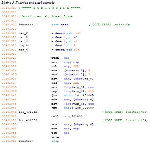
One of the most powerful aspects of IDA Pro is its ability to recognize functions, label them, and break down the local variables and parameters. Listing 5 shows an example of a function that has been recognized by IDA Pro. Notice how IDA Pro tells us that this is an EBP-based stack frame used in the function, which means the local variables and parameters will be referenced via the EBP register throughout the function. IDA Pro has successfully discovered all local variables and parameters in this function. It has labeled the local variables with the prefix var_ and parameters with the prefix arg_, and named the local variables and parameters with a suffix corresponding to their offset relative to EBP. IDA Pro will label only the local variables and parameters that are used in the code, and there is no way for you to know automatically if it has found everything from the original source code. Local variables will be at a negative offset relative to EBP and arguments will be at
a positive offset. You can see that IDA Pro has supplied the start of the summary of the stack view. The first line of this summary tells us that var_C corresponds to the value -0xCh. This is IDA Pro’s way of telling us that it has substituted var_C for -0xC; it has abstracted an instruction. For example, instead of needing to read the instruction as mov [ebp-0Ch], 3, we can simply read it as “var_C is now set to 3” and continue with our analysis.This abstraction makes reading the disassembly more efficient.

Sometimes IDA Pro will fail to identify a function. If this happens, you can create a function by pressing P. It may also fail to identify EBP-based stack frames, and the instructions mov [ebp-0Ch], eax and push dword ptr [ebp-010h] might appear instead of the convenient labeling. In most cases, you can fix this by pressing ALT-P, selecting BP Based Frame, and specifying 4 bytes for Saved Registers.
Using Graphing Options
IDA Pro supports five graphing options, accessible from the buttons on the toolbar shown in Figure 7. Four of these graphing options utilize cross-references. When you click one of these buttons on the toolbar, you will be presented with a graph via an application called WinGraph32. Unlike the graph view of the disassembly window, these graphs cannot be manipulated with IDA. (They are often referred to as legacy graphs.) The options on the graphing button toolbar are described in Table 1.

Enhancing Disassembly
One of IDA Pro’s best features is that it allows you to modify its disassembly to suit your goals. The changes that you make can greatly increase the speed with which you can analyze a binary.
Renaming Locations
IDA Pro does a good job of automatically naming virtual address and stack variables, but you can also modify these names to make them more meaningful. Auto-generated names (also known as dummy names) such as sub_401000 don’t tell you much; a function named ReverseBackdoorThread would be a lot more useful. You should rename these dummy names to something more meaningful. This will also help ensure that you reverse-engineer a function only once. When renaming dummy names, you need to do so in only one place. IDA Pro will propagate the new name wherever that item is referenced.

After you’ve renamed a dummy name to something more meaningful, cross-references will become much easier to parse. For example, if a function sub_401200 is called many times throughout a program and you rename it to DNSrequest, it will be renamed DNSrequest throughout the program. Imagine how much time this will save you during analysis, when you can read the meaningful name instead of needing to reverse the function again or to remember what sub_401200 does.

Table 2 shows an example of how we might rename local variables and arguments. The left column contains an assembly listing with no arguments renamed, and the right column shows the listing with the arguments renamed. We can actually glean some information from the column on the right. Here, we have renamed arg_4 to port_str and var_598 to port. You can see that these renamed elements are much more meaningful than their dummy names.

Comments
IDA Pro lets you embed comments throughout your disassembly and adds many comments automatically.
To add your own comments, place the cursor on a line of disassembly and press the colon (:) key on
your keyboard to bring up a comment window. To insert a repeatable comment to be echoed across the disassembly window whenever there is a cross-reference to the address in which you added the comment, press the semicolon (;) key.
Formatting Operands
When disassembling, IDA Pro makes decisions regarding how to format operands for each instruction that it disassembles. Unless there is context, the data displayed is typically formatted as hex values. IDA Pro allows you to change this data if needed to make it more understandable.
Figure 10 shows an example of modifying operands in an instruction, where 62h is compared to the local variable var_4. If you were to right-click 62h, you would be presented with options to change the 62h into 98 in decimal, 142o in octal, 1100010b in binary, or the character b in ASCII – whatever suits your needs and your situation.

To change whether an operand references memory or stays as data, press the O key on your keyboard.
For example, suppose when you’re analyzing disassembly with a link to loc_410000, you trace the link back and see the following instructions:
mov eax, loc_410000
add ebx, eax
mul ebx
At the assembly level, everything is a number, but IDA Pro has mislabeled the number 4259840 (0x410000 in hex) as a reference to the address 410000. To correct this mistake, press the O key to change this address to the number 410000h and remove the offending cross-reference from the disassembly window.
Using Named Constants
Malware authors (and programmers in general) often use named constants such as GENERIC_READ
in their source code. Named constants provide an easily remembered name for the programmer, but they are implemented as an integer in the binary. Unfortunately, once the compiler is done with the source code,it is no longer possible to determine whether the source used a symbolic constant or a literal.
Fortunately, IDA Pro provides a large catalog of named constants for the Windows API and the C standard library, and you can use the Use Standard Symbolic Constant option (shown in Figure 10) on an operand in your disassembly. Figure 11 shows the window that appears when you select Use Standard Symbolic Constant on the value 0x800000000.

The code snippets in Table 3 show the effect of applying the standard symbolic constants for a Windows API call to CreateFileA. Note how much more meaningful the code is on the right.

Sometimes a particular standard symbolic constant that you want will not appear, and you will need to load the relevant type library manually. To do so, select View→Open Subviews→Type Libraries to view the currently loaded libraries. Normally, mssdk and vc6win will automatically be loaded, but if not, you can load them manually (as is often necessary with malware that uses the Native API, the Windows NT family API). To get the symbolic constants for the Native API, load ntapi (the Microsoft Windows NT 4.0 Native API). In the same vein, when analyzing a Linux binary, you may need to manually load the gnuunx (GNU C++ UNIX) libraries.
Table 4. Manually Disassembling Shellcode in the paycuts.pdf Document

Redefining Code and Data
When IDA Pro performs its initial disassembly of a program, bytes are occasionally categorized incorrectly; code may be defined as data, data defined as code, and so on. The most common way to redefine code in the disassembly window is to press the U key to undefine functions, code, or data. When you undefine code, the underlying bytes will be reformatted as a list of raw bytes. To define the raw bytes as code, press C. For example, Table 4 shows a malicious PDF document named paycuts.pdf. At offset 0x8387 into the file, we discover shellcode (defined as raw bytes), so we press C at that location. This disassembles the shellcode and allows us to discover that it contains an XOR decoding loop with 0x97.
Depending on your goals, you can similarly define raw bytes as data or ASCII strings by pressing D or A, respectively.
The Interactive Disassembler Professional (IDA Pro) is an extremely powerful disassembler
distributed by Hex-Rays. Although IDA Pro is not the only disassembler, it is the disassembler
of choice for many malware analysts, reverse engineers, and vulnerability analysts.
The program is published by Hex-Rays (http://www.hex-rays.com), which provides a free version for noncommercial uses that is one version less than the current paid version. It is now version 5.0.
IDA Pro will disassemble an entire program and perform tasks such as function discovery, stack analysis, local variable identification, and much more. IDA Pro includes extensive code signatures within its Fast Library Identification and Recognition Technology (FLIRT), which allows it to recognize and label a disassembled function, especially library code added by a compiler.
IDA Pro is meant to be interactive, and all aspects of its disassembly process can be modified, manipulated, rearranged, or redefined. One of the best aspects of IDA Pro is its ability to save your analysis progress: You can add comments, label data, and name functions, and then save your work in an IDA Pro database (known as an idb) to return to later. IDA Pro also has robust support for plug-ins, so you can write your own extensions or leverage the work of others.
Loading an Executable
When you load an executable, IDA Pro will try to recognize the file’s format and processor architecture.Figure 1 displays the first step in loading an executable into IDA Pro. When loading a file into IDA Pro (such as a PE file with Intel x86 architecture), the program maps the file into memory as if it had been loaded by the operating system loader. To have IDA Pro disassemble the file as a raw binary, choose the Binary File option in the top box. This option can prove useful because malware sometimes appends shellcode, additional data, encryption parameters, and even additional executables to legitimate PE files, and this extra data won’t be loaded into memory when the malware is run by Windows or loaded into IDA Pro. In addition, when you are loading a raw binary file containing shellcode, you should choose to load the file as a binary file and disassemble it.
PE files are compiled to load at a preferred base address in memory, and if the Windows loader
can’t load it at its preferred address (because the address is already taken), the loader will perform
an operation known as rebasing. This most often happens with DLLs, since they are often loaded
at locations that differ from their preferred address. You should know that if you encounter a DLL loaded into a process different from what you see in IDA Pro, it could be the result of the file being rebased. When this occurs, check the Manual Load checkbox shown in Figur e 1, and you’ll see an input box where you can specify the new virtual base address in which to load the file.
By default, IDA Pro does not include the PE header or the resource sections in its disassembly (places where malware often hides malicious code). If you specify a manual load, IDA Pro will ask if you want to load each section, one by one, including the PE file header, so that these sections won’t escape analysis.
The IDA Pro Interface
After you load a program into IDA Pro, you will see the disassembly window, as shown in Figure 2. This will be your primary space for manipulating and analyzing binaries, and it’s where the assembly code resides.
Disassembly Window Modes
You can display the disassembly window in one of two modes: graph (the default, shown in Figure 2)
and text. To switch between modes, press the spacebar.
Graph Mode
In graph mode, IDA Pro excludes certain information that we recommend you display, such as line numbers and operation codes. To change these options, select Options→General, and then select Line prefixes and set the Number of Opcode Bytes to 6. Because most instructions contain 6 or fewer bytes, this setting will allow you to see the memory locations and opcode values for each instruction in the code listing (If these settings make everything scroll off the screen to the right, try setting the Instruction Indentation to 8).
In graph mode, the color and direction of the arrows help show the program’s flow during analysis.
The arrow’s color tells you whether the path is based on a particular decision having been made: red if a conditional jump is not taken, green if the jump is taken, and blue for an unconditional jump. The arrow direction shows the program’s flow; upward arrows typically denote a loop situation. Highlighting text in graph mode highlights every instance of that text in the disassembly window.
Text Mode
The text mode of the disassembly window is a more traditional view, and you must use it to view data
regions of a binary. Figure 3 displays the text mode view of a disassembled function. It displays the memory address (0040105B) and section name (.text) in which the opcodes (83EC18) will reside in memory.
The left portion of the text-mode display is known as the arrows window and shows the program’s nonlinear flow. Solid lines mark unconditional jumps, and dashed lines mark conditional jumps. Arrows facing up indicate a loop. The example includes the stack layout for the function and a comment (beginning with a semicolon) that was automatically added by IDA Pro.
Useful Windows for Analysis
Several other IDA Pro windows highlight particular items in an executable. The following are the most significant for our purposes.
Functions window Lists all functions in the executable and shows the length of each. You can sort by
function length and filter for large, complicated functions that are likely to be interesting, while excluding tiny functions in the process. This window also associates flags with each function (F, L, S, and so on), the most useful of which, L, indicates library functions. The L flag can save you time during analysis, because you can identify and skip these compiler-generated functions.
Names window Lists every address with a name, including functions, named code, named data, and strings.
Strings window Shows all strings. By default, this list shows only ASCII strings longer than five characters. You can change this by right-clicking in the Strings window and selecting Setup.
Imports window Lists all imports for a file.
Exports window Lists all the exported functions for a file. This window is useful when you’re analyzing DLLs.
Structures window Lists the layout of all active data structures. The window also provides you the ability to create your own data structures for use as memory layout templates.
These windows also offer a cross-reference feature that is particularly useful in locating interesting code. For example, to find all code locations that call an imported function, you could use the import window, doubleclick the imported function of interest, and then use the cross-reference feature to locate the import call in the code listing.
Returning to the Default View
The IDA Pro interface is so rich that, after pressing a few keys or clicking something, you may find it
impossible to navigate. To return to the default view, choose Windows→Reset Desktop. Choosing this option won’t undo any labeling or disassembly you’ve done; it will simply restore any windows and GUI elements to their defaults.
By the same token, if you’ve modified the window and you like what you see, you can save the new view by selecting Windows→Save desktop.
Navigating IDA Pro
As we just noted, IDA Pro can be tricky to navigate. Many windows are linked to the disassembly window. For example, double-clicking an entry within the Imports window or Strings window will take you directly to that entry.
Using Links and Cross-References
Another way to navigate IDA Pro is to use the links within the disassembly window, such as the links shown in Listing 1. Double-clicking any of these links will display the target location in the disassembly window. The following are the most common types of links:
• Sub links are links to the start of functions such as printf and sub_4010A0.
• Loc links are links to jump destinations such as loc_40107E and loc_401097.
• Offset links are links to an offset in memory.
Cross-references are useful for jumping the display to the referencing location: 0x401075 in this example. Because strings are typically references, they are also navigational links. For example, aPrintNumberD can be used to jump the display to where that string is defined in memory.
Exploring Your History
IDA Pro’s forward and back buttons, shown in Figure 4, make it easy to move through your history, just as you would move through a history of web pages in a browser. Each time you navigate to a new location within the disassembly window, that location is added to your history.
Navigation Band
The horizontal color band at the base of the toolbar is the navigation band, which presents a color-coded linear view of the loaded binary’s address space. The colors offer insight into the file contents at that location in the file as follows:
• Light blue is library code as recognized by FLIRT.
• Red is compiler-generated code.
• Dark blue is user-written code.
You should perform malware analysis in the dark-blue region. If you start getting lost in messy code,
the navigational band can help you get back on track. IDA Pro’s default colors for data are pink for imports, gray for defined data, and brown for undefined data.
Jump to Location
To jump to any virtual memory address, simply press the G key on your keyboard while in the disassembly window. A dialog box appears, asking for a virtual memory address or named location, such as sub_401730 or printf.
Listing 1. Navigational links within the disassembly window
00401075 jnz short loc_40107E
00401077 mov [ebp+var_10], 1
0040107E loc_40107E: ; CODE XREF: sub_401040+35j
0040107E cmp [ebp+var_C], 0
00401082 jnz short loc_401097
00401084 mov eax, [ebp+var_4]
00401087 mov [esp+18h+var_14], eax
0040108B mov [esp+18h+var_18], offset aPrintNumberD ; “Print Number= %d\n”
00401092 call printf
00401097 call sub_4010A0
To jump to a raw file offset, choose Jump→Jump to File Offset. For example, if you’re viewing a PE file in a hex editor and you see something interesting, such as a string or shellcode, you can use this feature to get to that raw offset, because when the file is loaded into IDA Pro, it will be mapped as though it had been loaded by the OS loader.
Searching
Selecting Search from the top menu will display many options for moving the cursor in the disassembly window:
• Choose Search→Next Code to move the cursor to the next location containing an instruction you specify.
• Choose Search→Text to search the entire disassembly window for a specific string.
• Choose Search→Sequence of Bytes to perform a binary search in the hex view window for a certain byte order. This option can be useful when you’re searching for specific data or opcode combinations.
The following example displays the command-line analysis of the password.exe binary. This malware
requires a password to continue running, and you can see that it prints the string Bad key after we enter an invalid password (test).
C:\>password.exe
Enter password for this Malware: test
Bad key
We then pull this binary into IDA Pro and see how we can use the search feature and links to unlock the program. We begin by searching for all occurrences of the Bad key string, as shown in Figure 5. We notice that Bad key is used at 0x401104, so we jump to that location in the disassembly window by double-clicking the entry in the search window.
Listing 2. The disassembly listing
004010E0 push offset aMab ; “$mab”
004010E5 lea ecx, [ebp+var_1C]
004010E8 push ecx
004010E9 call strcmp
004010EE add esp, 8
004010F1 test eax, eax
004010F3 jnz short loc_401104
004010F5 push offset aKeyAccepted ; “Key Accepted!\n”
004010FA call printf
004010FF add esp, 4
00401102 jmp short loc_401118
00401104 loc_401104 ; CODE XREF: _main+53j
00401104 push offset aBadKey ; “Bad key\n”
00401109 call printf
The disassembly listing around the location of 0x401104 is shown next. Looking through the listing, before „Bad key\n”, we see a comparison at 0x4010F1, which tests the result of a strcmp. One of the parameters to the strcmp is the string, and likely password, $mab (Listing 2). The next example shows the result of entering the password we discovered, $mab, and the program prints a different result.
C:\>password.exe
Enter password for this Malware: $mab
Key Accepted!
The malware has been unlocked
This example demonstrates how quickly you can use the search feature and links to get information about a binary.
Using Cross-References
A cross-reference, known as an xref in IDA Pro, can tell you where a function is called or where a string is used. If you identify a useful function and want to know the parameters with which it is called, you can use a cross-reference to navigate quickly to the location where the parameters are placed on the stack. Interesting graphs can also be generated based on cross-references, which are helpful to performing analysis.
Code Cross-References
Listing 3 shows a code cross-reference that tells us that this function (sub_401000) is called from inside the main function at offset 0x3 into the main function. The code cross-reference for the jump tells us which jump takes us to this location, which in this example corresponds to the location marked at the end. We know this because at offset 0x19 into sub_401000 is the jmp at memory address 0x401019.
By default, IDA Pro shows only a couple of cross-references for any given function, even though many may occur when a function is called. To view all the cross-references for a function, click the function name and press X on your keyboard. The window that pops up should list all locations where this function is called. At the bottom of the Xrefs window in Figure 6, which shows a list of cross-references for sub_408980, you can see that this function is called 64 times (“Line 1 of 64”). Double-click any entry in the Xrefs window to go to the corresponding reference in the disassembly window.
Data Cross-References
Data cross-references are used to track the way data is accessed within a binary. Data references can be associated with any byte of data that is referenced in code via a memory reference, as shown in Listing 4. For example, you can see the data cross-reference to the DWORD 0x7F000001. The corresponding cross-reference tells us that this data is used in the function located at 0x401020. The following line shows a data crossreference for the string <Hostname> <Port>.
The static analysis of strings can often be used as a starting point for your analysis. If you see an interesting string, use IDA Pro’s cross-reference feature to see exactly where and how that string is used within the code.
Analyzing Functions
One of the most powerful aspects of IDA Pro is its ability to recognize functions, label them, and break down the local variables and parameters. Listing 5 shows an example of a function that has been recognized by IDA Pro. Notice how IDA Pro tells us that this is an EBP-based stack frame used in the function, which means the local variables and parameters will be referenced via the EBP register throughout the function. IDA Pro has successfully discovered all local variables and parameters in this function. It has labeled the local variables with the prefix var_ and parameters with the prefix arg_, and named the local variables and parameters with a suffix corresponding to their offset relative to EBP. IDA Pro will label only the local variables and parameters that are used in the code, and there is no way for you to know automatically if it has found everything from the original source code. Local variables will be at a negative offset relative to EBP and arguments will be at
a positive offset. You can see that IDA Pro has supplied the start of the summary of the stack view. The first line of this summary tells us that var_C corresponds to the value -0xCh. This is IDA Pro’s way of telling us that it has substituted var_C for -0xC; it has abstracted an instruction. For example, instead of needing to read the instruction as mov [ebp-0Ch], 3, we can simply read it as “var_C is now set to 3” and continue with our analysis.This abstraction makes reading the disassembly more efficient.
Sometimes IDA Pro will fail to identify a function. If this happens, you can create a function by pressing P. It may also fail to identify EBP-based stack frames, and the instructions mov [ebp-0Ch], eax and push dword ptr [ebp-010h] might appear instead of the convenient labeling. In most cases, you can fix this by pressing ALT-P, selecting BP Based Frame, and specifying 4 bytes for Saved Registers.
Using Graphing Options
IDA Pro supports five graphing options, accessible from the buttons on the toolbar shown in Figure 7. Four of these graphing options utilize cross-references. When you click one of these buttons on the toolbar, you will be presented with a graph via an application called WinGraph32. Unlike the graph view of the disassembly window, these graphs cannot be manipulated with IDA. (They are often referred to as legacy graphs.) The options on the graphing button toolbar are described in Table 1.
Enhancing Disassembly
One of IDA Pro’s best features is that it allows you to modify its disassembly to suit your goals. The changes that you make can greatly increase the speed with which you can analyze a binary.
Renaming Locations
IDA Pro does a good job of automatically naming virtual address and stack variables, but you can also modify these names to make them more meaningful. Auto-generated names (also known as dummy names) such as sub_401000 don’t tell you much; a function named ReverseBackdoorThread would be a lot more useful. You should rename these dummy names to something more meaningful. This will also help ensure that you reverse-engineer a function only once. When renaming dummy names, you need to do so in only one place. IDA Pro will propagate the new name wherever that item is referenced.
After you’ve renamed a dummy name to something more meaningful, cross-references will become much easier to parse. For example, if a function sub_401200 is called many times throughout a program and you rename it to DNSrequest, it will be renamed DNSrequest throughout the program. Imagine how much time this will save you during analysis, when you can read the meaningful name instead of needing to reverse the function again or to remember what sub_401200 does.
Table 2 shows an example of how we might rename local variables and arguments. The left column contains an assembly listing with no arguments renamed, and the right column shows the listing with the arguments renamed. We can actually glean some information from the column on the right. Here, we have renamed arg_4 to port_str and var_598 to port. You can see that these renamed elements are much more meaningful than their dummy names.
Comments
IDA Pro lets you embed comments throughout your disassembly and adds many comments automatically.
To add your own comments, place the cursor on a line of disassembly and press the colon (:) key on
your keyboard to bring up a comment window. To insert a repeatable comment to be echoed across the disassembly window whenever there is a cross-reference to the address in which you added the comment, press the semicolon (;) key.
Formatting Operands
When disassembling, IDA Pro makes decisions regarding how to format operands for each instruction that it disassembles. Unless there is context, the data displayed is typically formatted as hex values. IDA Pro allows you to change this data if needed to make it more understandable.
Figure 10 shows an example of modifying operands in an instruction, where 62h is compared to the local variable var_4. If you were to right-click 62h, you would be presented with options to change the 62h into 98 in decimal, 142o in octal, 1100010b in binary, or the character b in ASCII – whatever suits your needs and your situation.
To change whether an operand references memory or stays as data, press the O key on your keyboard.
For example, suppose when you’re analyzing disassembly with a link to loc_410000, you trace the link back and see the following instructions:
mov eax, loc_410000
add ebx, eax
mul ebx
At the assembly level, everything is a number, but IDA Pro has mislabeled the number 4259840 (0x410000 in hex) as a reference to the address 410000. To correct this mistake, press the O key to change this address to the number 410000h and remove the offending cross-reference from the disassembly window.
Using Named Constants
Malware authors (and programmers in general) often use named constants such as GENERIC_READ
in their source code. Named constants provide an easily remembered name for the programmer, but they are implemented as an integer in the binary. Unfortunately, once the compiler is done with the source code,it is no longer possible to determine whether the source used a symbolic constant or a literal.
Fortunately, IDA Pro provides a large catalog of named constants for the Windows API and the C standard library, and you can use the Use Standard Symbolic Constant option (shown in Figure 10) on an operand in your disassembly. Figure 11 shows the window that appears when you select Use Standard Symbolic Constant on the value 0x800000000.
The code snippets in Table 3 show the effect of applying the standard symbolic constants for a Windows API call to CreateFileA. Note how much more meaningful the code is on the right.
Sometimes a particular standard symbolic constant that you want will not appear, and you will need to load the relevant type library manually. To do so, select View→Open Subviews→Type Libraries to view the currently loaded libraries. Normally, mssdk and vc6win will automatically be loaded, but if not, you can load them manually (as is often necessary with malware that uses the Native API, the Windows NT family API). To get the symbolic constants for the Native API, load ntapi (the Microsoft Windows NT 4.0 Native API). In the same vein, when analyzing a Linux binary, you may need to manually load the gnuunx (GNU C++ UNIX) libraries.
Redefining Code and Data
When IDA Pro performs its initial disassembly of a program, bytes are occasionally categorized incorrectly; code may be defined as data, data defined as code, and so on. The most common way to redefine code in the disassembly window is to press the U key to undefine functions, code, or data. When you undefine code, the underlying bytes will be reformatted as a list of raw bytes. To define the raw bytes as code, press C. For example, Table 4 shows a malicious PDF document named paycuts.pdf. At offset 0x8387 into the file, we discover shellcode (defined as raw bytes), so we press C at that location. This disassembles the shellcode and allows us to discover that it contains an XOR decoding loop with 0x97.
Depending on your goals, you can similarly define raw bytes as data or ASCII strings by pressing D or A, respectively.